How FDA can vet dose-escalation trials for safety
David C. Norris
9/20/2020
Source:vignettes/FDA-proactive.Rmd
FDA-proactive.RmdBackground
Norris (2020) examines a fatal dose-finding trial (AFM11-102) in retrospect, through the lens of a somewhat realistic Bayesian model of ordinal toxicity outcomes. When this model is estimated using only data from the first 5 dose cohorts, it foresees as reasonably likely the fatal toxicity which actually occurred in the 6th cohort. Thus, even in this inherently unsafe trial, disaster might still have been averted through the dynamic ‘situational awareness’ a realistic model can deliver.
Unfortunately, realistic models of the kind employed in Norris (2020) are unlikely to be contemplated or even understood by trial sponsors who deploy 3+3 designs like the one in question. Indeed, even FDA’s Oncology Center of Excellence (OCE) expresses at best limited enthusiasm for early-phase trial designs that are cognizant of inter-individual heterogeneity. Thus, the question arises: would a less sophisticated analysis have enabled the sponsor, or FDA, to recognize this trial’s unsafe design from the outset?
Mapping the trial to the precautionary package
AFM11-102 used two modifications that do not map readily to designs implemented in the escalation package on which precautionary is based. Firstly, whereas the design specified an initial ‘accelerated titration’ phase (Simon et al. 1997), we will simply simulate a standard ‘3+3’ design.1 Secondly, the trial employed step-up dosing such that patients initiated treatment at 1/3 of their cohort’s target dose, stepping up to the full dose after 1 week. Whereas the abovementioned Bayesian model exploited the extra information available from this step-up protocol, we will for present purposes regard each cohort as characterized simply by its target dose:
library(precautionary)
design <- get_three_plus_three(num_doses = 6)
options(dose_levels = c(2, 6, 20, 60, 180, 400)) # ng/kg/week
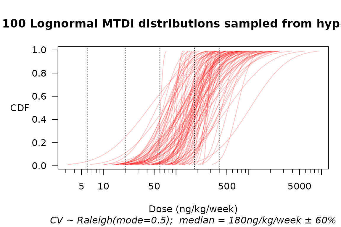
As in Norris (2020), we suppose \(\mathrm{MTD}_i\) is lognormally distributed, with a coefficient of variation (CV) of 1/2, and a median centered at the next-to-highest dose of 180 ng/kg/week. We allow for a ±60% uncertainty in this median.2
mtdi_gen <- hyper_mtdi_lognormal(CV = 0.5
                                ,median_mtd = 180
                                ,median_sdlog = 0.6
                                ,units="ng/kg/week"
                                )
plot(mtdi_gen, n=100, col=adjustcolor("red", alpha=0.25))
Multiple samples from a hyperprior over the distribution of MTD\(_i\).
Finally, we introduce a standard ‘ordinalizer’ that assumes the toxicity-grade thresholds for any individual patient are a geometric sequence of doses with ratio \(r_0\).3
Simulating safety
set.seed(2020)
design %>% simulate_trials(
  num_sims = 100
, true_prob_tox = mtdi_gen
) %>% extend(target_mcse = 0.1) -> SIMS
summary(SIMS,r0 = 2)$safety %>%
safety_kable() | None | Gr1 | Gr2 | Gr3 | Gr4 | Gr5 | Total |
|---|---|---|---|---|---|---|
| 9.9 | 2.1 | 2.3 | 1.8 | 0.6 | 0.1 | 16.9 |
Uncertainty about the ordinalizer
What about our uncertainty over the therapeutic index \(r_0\)? Here, it seems entirely reasonable simply to explore a range of values:
r0 <- seq(1.2, 2.0, 0.2); names(r0) <- format(r0, 2)
safetytabs <- sapply(r0, FUN = function(.) summary(SIMS, r0=.)$safety
                     , simplify = "array", USE.NAMES = TRUE)
cbind(data.table(`$r_0$` = r0), t(safetytabs[1,,])) %>%
  kable(digits=2) %>% add_header_above(
c(" "=1, "Expected counts by toxicity grade"=6, " "=1))| \(r_0\) | None | Gr1 | Gr2 | Gr3 | Gr4 | Gr5 | Total |
|---|---|---|---|---|---|---|---|
| 1.2 | 13.16 | 0.58 | 0.61 | 0.60 | 0.49 | 1.50 | 16.94 |
| 1.4 | 12.10 | 1.16 | 1.10 | 1.01 | 0.78 | 0.80 | 16.94 |
| 1.6 | 11.24 | 1.53 | 1.59 | 1.36 | 0.83 | 0.40 | 16.94 |
| 1.8 | 10.53 | 1.83 | 2.00 | 1.61 | 0.77 | 0.20 | 16.94 |
| 2.0 | 9.88 | 2.15 | 2.33 | 1.82 | 0.64 | 0.12 | 16.94 |
Focusing on the expected numbers of fatal toxicities, and with proper attention to Monte Carlo standard errors (MCSEs) of these expectations, we might tabulate as follows:
cbind(data.table(`$r_0$` = r0), t(safetytabs[,'Gr5',])) %>%
  kable(digits=2,
        col.names = c('$r_0$',
                      'Expected fatal toxicities',
                      'MCSE')) %>%
kable_styling(full_width = FALSE, position = "left")| \(r_0\) | Expected fatal toxicities | MCSE |
|---|---|---|
| 1.2 | 1.50 | 0.05 |
| 1.4 | 0.80 | 0.04 |
| 1.6 | 0.40 | 0.03 |
| 1.8 | 0.20 | 0.02 |
| 2.0 | 0.12 | 0.02 |
Applying the simulation results
Safety parameters for any given phase 1 trial necessarily depend on the clinical context and unmet need addressed by the investigational drug (Muller and Milton 2012). For sake of discussion, suppose FDA would have required an expected probability of any fatality in AFM11-102 to be below 15%. Then FDA might have requested that the sponsor support an expectation that \(r_0 > 2\) (e.g., based on preclinical evidence), or else modify the trial design.
References
Muller, Patrick Y., and Mark N. Milton. 2012. “The Determination and Interpretation of the Therapeutic Index in Drug Development.” Nature Reviews. Drug Discovery 11 (10): 751–61. https://doi.org/10.1038/nrd3801.
Norris, David C. 2020. “Retrospective Analysis of a Fatal Dose-Finding Trial.” arXiv:2004.12755 [stat.ME], April. https://arxiv.org/abs/2004.12755.
Simon, R., B. Freidlin, L. Rubinstein, S. G. Arbuck, J. Collins, and M. C. Christian. 1997. “Accelerated Titration Designs for Phase I Clinical Trials in Oncology.” Journal of the National Cancer Institute 89 (15): 1138–47. https://doi.org/10.1093/jnci/89.15.1138.
Note that omitting the accelerated titration makes our simulated trial safer, thus biasing our analysis toward a finding of safety.↩︎
That is, \(\log(median) \sim \mathscr{N}(\log 180, 0.6)\).↩︎
With our focus being safety, it is important mainly that these dose ratios hold between the higher grades, linking Grades 3–4, and Grades 4–5.↩︎