Introduction to package 'precautionary' • precautionary

Basics

In package escalation, you can simulate a 3 + 3 design as follows:

library(escalation)
# Design a 3 + 3 trial, with 5 prespecified doses to escalate through
design <- get_three_plus_three(num_doses = 5)
# Posit a scenario where these 5 doses cause dose-limiting toxicities
# (DLTs) in 12%, 27%, etc. of the population:
scenario <- c(0.12, 0.27, 0.44, 0.53, 0.57)
design %>% simulate_trials( # Feed the design to the simulator ...
  num_sims = 100            # run 100 simulated trials
, true_prob_tox = scenario  # under the chosen scenario,
) -> sims                   # and store the results.

summary(sims) # summarize simulation results

Simulation summary as produced by package `escalation`.
dose	tox	n	true_prob_tox	prob_recommend	prob_administer
NoDose	0.00	0.00	0.00	0.11	0.0000000
1	0.48	4.02	0.12	0.41	0.3806818
2	1.03	3.87	0.27	0.36	0.3664773
3	0.99	2.04	0.44	0.10	0.1931818
4	0.26	0.51	0.53	0.02	0.0482955
5	0.08	0.12	0.57	0.00	0.0113636

From Table @ref(tab:basic-sim), we learn a few things of interest. For example, we see that, with the lowest dose being too toxic for 12% of the population, under this scenario there is a real chance even this dose will be rejected by our trial. Conversely, we also find it is not impossible for our trial to recommend a dose that is toxic to nearly half the population. Note also that, by summing the \(n\) column, we can estimate expected enrollment at 10.56, which perhaps informs us about the expected cost or duration of our trial.¹

But simulations such as these cannot answer crucial questions about trial safety, mainly because the simulation machinery recognizes no notion of graded toxicity. The binary (yes/no) toxicities in the simulation machinery of escalation regard Grade 5 (fatal) toxicities no differently from Grade 3.

Introducing realistic pharmacologic thinking

The precautionary package solves this problem by pursuing a realistic approach to pharmacologic thinking. Rather than plucking a sequence of toxicity probabilities out of thin air, this approach derives such probabilities according to how a latent toxicity threshold is distributed in the population.

library(precautionary)
mtdi_dist <- mtdi_lognormal(CV = 2          # coefficient of variation
                           ,median = 5      # median DLT threshold
                           ,units = "mg/kg" # real doses have units!
                           )

Likewise, the prespecified doses for our dose-escalation design must be specified as actual doses. With package precautionary, this is accomplished by setting a dose_levels option:

options(dose_levels = c(0.5, 1, 2, 4, 6)) # specify actual dosing

A plot of the \(\mathrm{MTD}_i\) distribution makes clear the connection with toxicity probabilities:

plot(mtdi_dist)

probs <- mtdi_dist@dist$cdf(getOption('dose_levels'))
names(probs) <- paste(getOption('dose_levels'), mtdi_dist@units)
t(probs) %>% kable(digits = 4)

0.5 mg/kg	1 mg/kg	2 mg/kg	4 mg/kg	6 mg/kg
0.0348	0.1023	0.2351	0.4302	0.5571

Extending `escalation` to support the \(\mathrm{MTD}_i\) concept

Package precautionary provides additional methods for escalation functions, so that an mtdi_distribution may be used instead of out-of-thin-air probabilities:

design %>% simulate_trials(
  num_sims = 100
, true_prob_tox = mtdi_dist # pull tox probs from a MODEL, not thin air
) -> SIMS

summary(SIMS)

A simulation summary under the MTD\(_i\) regime of package `precautionary`.
dose	dose (mg/kg)	tox	n	true_prob_tox	prob_recommend	prob_administer
NoDose	0.0	0.00	0.00	0.0000000	0.00	0.0000000
1	0.5	0.04	3.12	0.0347613	0.14	0.2369021
2	1.0	0.40	3.54	0.1022854	0.37	0.2687927
3	2.0	1.00	3.87	0.2350660	0.36	0.2938497
4	4.0	0.88	2.04	0.4301892	0.13	0.1548975
5	6.0	0.33	0.60	0.5571371	0.00	0.0455581

Judging from Table @ref(tab:MTDi-regime), however, introducing the \(\mathrm{MTD}_i\) concept has by itself generated little progress. The only apparent improvement compared with Table @ref(tab:basic-sim) is the addition of a column with actual doses. To make further progress while continuing to operate within the dose-escalation paradigm, we need to introduce another concept.

Introducing graded toxicities

When its full implications are allowed to develop, the latent toxicity threshold \(\mathrm{MTD}_i\) has far-reaching consequences for the design of dose-finding trials. Indeed, it forms the conceptual basis for dose-titration designs that abandon cohortwise dose-escalation altogether (Norris 2017a, 2017b).

For present purposes, however, we take it for granted that (for whatever reason) we have chosen to employ a dose-escalation design. That choice effectively discards the core insight of \(\mathrm{MTD}_i\), and relegates the \(\mathrm{MTD}_i\) concept standing alone to the status of a mere formalism. But in conjunction with a dose scaling that links different toxicity grades at the individual level, the \(\mathrm{MTD}_i\) can be rehabilitated as an effective tool, even within the confines of a dose-escalation design. In package precautionary, such scaling functions are called ‘ordinalizers’, and may be applied at the time when simulations are summarized:

tox_threshold_scaling <- function(MTDi, r0) {
  MTDi * r0 ^ c(Gr1=-2, Gr2=-1, Gr3=0, Gr4=1, Gr5=2)
}
summary(SIMS
       ,ordinalizer = tox_threshold_scaling
       ,r0 = 2      # supply a value for ordinalizer's r0 parameter
       )$safety %>% # select the 'safety' component of the summary
  safety_kable()

Expected counts per toxicity grade
None	Gr1	Gr2	Gr3	Gr4	Gr5	Total
6	2	2	1.4	0.8	0.5	13

Clearly, we have now made some genuine progress. Of special interest from a safety perspective are the numbers of Grade 4 (severe) and Grade 5 (fatal) toxicities expected in the trial.

A closer look at the ordinalizer

Let us unroll the ordinalizer above, to make it less cryptic:

tox_threshold_scaling <-
  function(MTDi   # An ordinalizer is a function of a dose threshold,
          ,r0 = 2 # and in general has additional parameters as well.
          ) {
    # An ordinalizer assumes we start with a binary toxicity notion,
    # and maps that to a *graded* notion of toxicity by means of a
    # transformation in 'dose-space'.
    # Assuming the default value r0 = 2 provided in its definition,
    # this ordinalizer says that an individual whose dose threshold
    # for the binary toxicity is MTDi has thresholds ...
    c(Gr1 = MTDi / r0^2 # at MTDi/4 for Gr1,
     ,Gr2 = MTDi / r0   # at MTDi/2 for Gr2,
     ,Gr3 = MTDi        # at MTDi for Gr3 ('tox' is defined as Gr3+),
     ,Gr4 = MTDi * r0   # at 2*MTDi for Gr4,
     ,Gr5 = MTDi * r0^2 # at 4*MTDi for Gr5.
    )
  }

In general, an ordinalizer returns a named vector² that links the different dose thresholds at which an individual will experience each grade of toxicity. In (Norris 2020), these concepts are laid out in terms of \(\mathrm{MTD}_i^{g}\) with the index \(g\) running over toxicity grades:

\[ \mathrm{MTD}_i^{g}, g \in \{1,...,5\}, \]

and defined as the dose threshold where a grade-\((g-1)\) toxicity would convert to grade-\(g\).³ Thus, in the usual case where the binary ‘dose-limiting toxicity’ (DLT) of a dose-escalation design is defined as CTCAE Grade ≥ 3, we identify ‘\(\mathrm{MTD}_i\)’ with \(\mathrm{MTD}_i^{3}\) .

Taking stock of parameter counts

It might seem that the benefits of package precautionary come at the cost of having to prespecify many additional parameters. Au contraire! In the example above, the CV and median parameters of mtdi_dist replaced the 5 ‘true toxicity probabilities’ that the package-escalation approach requires you to pluck out of thin air. Thus, immediately we have saved 3 parameters. From this savings, we then spent only 1 on the single parameter r0 of our simple ordinalizer. Indeed, if we had wished to spend all of our ‘parameter savings’, we could have specified an ordinalizer such as:⁴

function(MTDi3, r12, r4, r5) {
  c(Gr1 = MTDi3 / r12^2
   ,Gr2 = MTDi3 / r12
   ,Gr3 = MTDi3
   ,Gr4 = MTDi3 * r4
   ,Gr5 = MTDi3 * r4*r5
   )
}

As we count design parameters, we also ought not overlook the prespecified dose levels themselves, which are indeed parameters of our design. But package precautionary changes the manner in which these parameters enter into simulation-based trial design. In the usual approach, every new set of prespecified dose levels requires its own set of ‘true toxicity probabilities’ to be pulled anew out of thin air. But in package precautionary, the linkage between dose levels and probabilities is provided through a model. In theory, this would allow us to obtain our dose levels as results of simulation-based design, instead of providing them as inputs.

Modeling uncertainty

When you ask people to start thinking, sometimes they keep going. No sooner will you have elicited values for the CV and median parametrizing a lognormal \(\mathrm{MTD}_i\) distribution

\[ \begin{align} \log \mathrm{MTD}_i &\sim \mathscr{N}(\mu, \sigma^2) \\ \mu &\equiv \log(\mathrm{median}) \\ \sigma^2 &\equiv \log (1+\mathrm{CV}^2), \end{align} \]

than you will hear about the uncertainty in these values themselves. You can model this uncertainty by introducing hyperparameters \(\sigma_{\mathrm{CV}}\) and \(\sigma_{\mathrm{med}}\):

\[ \begin{align} \mu &\sim \mathscr{N}(\log \mathrm{median}, \sigma_{\mathrm{med}}^2) \\ \mathrm{CV} &\sim \mathscr{R}(\sigma_{\mathrm{CV}}) \end{align} \]

Here, \(\sigma_{\mathrm{med}}\) expresses in relative terms⁵ our uncertainty about the median of \(\mathrm{MTD}_i\), while \(\sigma_{\mathrm{CV}}\) is the parameter of the Raleigh distribution:

Happily, the Raleigh distribution’s \(\sigma\) parameter coincides with its mode (likeliest value), and its standard deviation is about \(\frac{2}{3} \sigma\), which seems a reasonable degree of relative uncertainty about CV(\(\mathrm{MTD}_i\)).⁶ We take advantage of this when we implement these features in package precautionary, avoiding the need to ask users to specify a separate uncertainty parameter for CV:

mtdi_gen <- hyper_mtdi_lognormal(CV = 1
                                ,median_mtd = 5
                                ,median_sdlog = 0.5 # this is new
                                ,units="mg/kg"
                                )
plot(mtdi_gen, n=100, col=adjustcolor("red", alpha=0.25))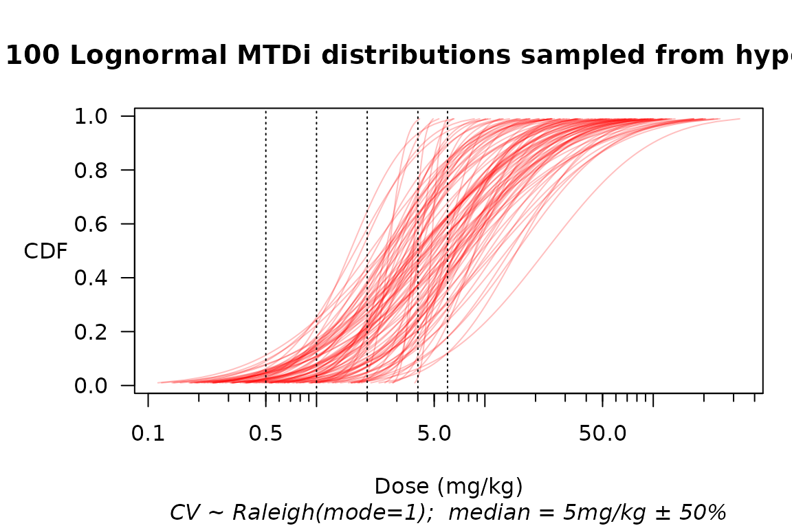

Multiple samples from a hyperprior over the distribution of MTD\(_i\). Consider the implications for the customary practice of pulling ‘true toxicity probabilities’ out of thin air!

design %>% simulate_trials(
  num_sims = 400
, true_prob_tox = mtdi_gen # pull tox probs from MANY models
) -> HYPERSIMS

# As a convenience, package 'precautionary' lets you set the
# ordinalizer as an *option* so that you don't have to keep
# specifying it as an argument to summary(). By providing a
# default setting for the r0 parameter in the ordinalizer
# definition, we avoid having to keep specifying that, too.
options(ordinalizer = function(MTDi, r0 = 1.5) {
  MTDi * r0 ^ c(Gr1=-2, Gr2=-1, Gr3=0, Gr4=1, Gr5=2)
})

summary(HYPERSIMS)$safety

Expected counts per toxicity grade
None	Gr1	Gr2	Gr3	Gr4	Gr5	Total
9	1.8	1.6	1.1	0.6	0.7	15

Uncertainty about the ordinalizer

What about our uncertainty over the parameter \(r_0\)? Here, it seems entirely reasonable simply to explore a range of values:

r0 <- c(1.25, 1.5, 1.75, 2.0)
rbind(summary(HYPERSIMS, r0=r0[1])$safety[1,]
     ,summary(HYPERSIMS, r0=r0[2])$safety[1,]
     ,summary(HYPERSIMS, r0=r0[3])$safety[1,]
     ,summary(HYPERSIMS, r0=r0[4])$safety[1,]
     ) -> safety
cbind(data.table(`$r_0$` = r0), safety) %>% kable(digits=2) %>%
  add_header_above(c(" "=1, "Expected counts by toxicity grade"=6, " "=1))

	Expected counts by toxicity grade
\(r_0\)	None	Gr1	Gr2	Gr3	Gr4	Gr5	Total
1.25	10.33	0.97	0.80	0.64	0.53	1.27	14.54
1.50	8.74	1.78	1.57	1.08	0.64	0.72	14.54
1.75	7.38	2.50	2.22	1.37	0.68	0.40	14.54
2.00	6.30	2.94	2.86	1.57	0.62	0.26	14.54

Beyond 3 + 3

One reason that package escalation makes such a suitable basis for these developments is that it unifies several dose-escalation designs under one object-oriented design. Thus, we can repeat the above simulation exercise with a CRM design:

crm_design <- get_dfcrm(skeleton = scenario, target = 0.25) %>%
  stop_at_n(n = 24)
crm_design %>% simulate_trials(
  num_sims = 200
, true_prob_tox = mtdi_gen
) -> CRM_HYPERSIMS

summary(CRM_HYPERSIMS)$safety

Expected counts per toxicity grade
None	Gr1	Gr2	Gr3	Gr4	Gr5	Total
12	4	3	2	1.3	1.4	24.0

The BOIN design of (Liu and Yuan 2015) is also supported:

boin_design <- get_boin(num_doses = 5, target = 0.25) %>%
  stop_at_n(n = 24)
boin_design %>% simulate_trials(
  num_sims = 200
, true_prob_tox = mtdi_gen
) -> BOIN_HYPERSIMS

summary(BOIN_HYPERSIMS)$safety

Expected counts per toxicity grade
None	Gr1	Gr2	Gr3	Gr4	Gr5	Total
13	3	3	2.0	1.1	1.1	24.0

Implications of package `precautionary`

Package precautionary demonstrates in principle that any dose-escalation design can be assessed for safety, given a modicum of realistic pharmacologic thinking during prior elicitation. How truly modest this additional input is, should be apparent from the obvious connections between the ratios in an ‘ordinalizer’ and the notion of therapeutic index (TI). It is hard to imagine that any trialist would pursue a phase 1 investigation without some notion of a plausible range for TI (Muller and Milton 2012). Yet within the biostatistical literature on dose-finding methods, I know of no attempt to apply a TI concept formally to assess design safety.

References

Liu, Suyu, and Ying Yuan. 2015. “Bayesian Optimal Interval Designs for Phase I Clinical Trials.” Journal of the Royal Statistical Society: Series C (Applied Statistics) 64 (3): 507–23. https://doi.org/10.1111/rssc.12089.

Muller, Patrick Y., and Mark N. Milton. 2012. “The Determination and Interpretation of the Therapeutic Index in Drug Development.” Nature Reviews. Drug Discovery 11 (10): 751–61. https://doi.org/10.1038/nrd3801.

Norris, David C. 2017a. “Dose Titration Algorithm Tuning (DTAT) Should Supersede ‘the’ Maximum Tolerated Dose (MTD) in Oncology Dose-Finding Trials.” F1000Research 6 (July): 112. https://doi.org/10.12688/f1000research.10624.3.

———. 2017b. “Precautionary Coherence Unravels Dose Escalation Designs.” bioRxiv, December. https://doi.org/10.1101/240846.

———. 2020. “Retrospective Analysis of a Fatal Dose-Finding Trial.” arXiv:2004.12755 [stat.ME], April. https://arxiv.org/abs/2004.12755.

Any complete simulation study will of course consider multiple scenarios, perhaps weighted according to their varying likelihood.↩︎
The names allow for user-customized labeling of the toxicity levels, which carries forward into summaries, etc.↩︎
To preserve the intuition of the term ‘maximum tolerated dose’, you could say \(\mathrm{MTD}_i^{g}\) is the maximum dose that individual \(i\) can tolerate if ‘tolerability’ is defined as toxicity below grade-\(g\).↩︎
Note the judicious allocation of parameters. This ordinalizer devotes 2 parameters (r4 and r5) to the safety-critical threshold ratios \(r_4 := \mathrm{MTD}_i^3 : \mathrm{MTD}_i^4\) and \(r_5 := \mathrm{MTD}_i^3 : \mathrm{MTD}_i^4\), but conserves on parameters by sharing the same parameter \(r_{12}\) for the ratios involving low-grade toxicities.↩︎
For example, setting \(\sigma_{\mathrm{med}} = 0.5\) would express a ±50% uncertainty in our guessed median \(\mathrm{MTD}_i\).↩︎
The exact figure is \(\sqrt{2-\pi/2} \approx 0.655\). Given how little is known generally—or even acknowledged!—about inter-individual variation in optimal dosing, it seems reasonable to suppose that you will allow a ± of 66% on any value you choose as most likely for \(\mathrm{CV}(\mathrm{MTD}_i)\).↩︎

Introduction to package ‘precautionary’

David C. Norris

7/31/2020

Basics

Introducing realistic pharmacologic thinking

Extending `escalation` to support the \(\mathrm{MTD}_i\) concept

Introducing graded toxicities

A closer look at the ordinalizer

Taking stock of parameter counts

Modeling uncertainty

Uncertainty about the ordinalizer

Beyond 3 + 3

Implications of package `precautionary`

References

Introduction to package ‘precautionary’

David C. Norris

7/31/2020

Basics

Introducing realistic pharmacologic thinking

Extending escalation to support the \(\mathrm{MTD}_i\) concept

Introducing graded toxicities

A closer look at the ordinalizer

Taking stock of parameter counts

Modeling uncertainty

Uncertainty about the ordinalizer

Beyond 3 + 3

Implications of package precautionary

References

Extending `escalation` to support the \(\mathrm{MTD}_i\) concept

Implications of package `precautionary`